

1.
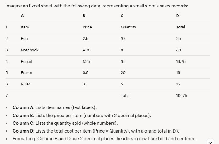
How was the value 25 in cell D2 calculated using the data in the sheet?
2.
What function can you use to verify that the grand total in D7 (112.75) is correct?
3.
Which function would tell you the highest quantity sold from column C, and what is the result?
4.
If a 5% discount rate is in cell B8, how would you calculate the discounted total for Pens in E2, ensuring the discount rate stays fixed when copied?
5.
How would you create a column chart to compare the total sales of each item, and what data range would you select?
1.
Answer: It was calculated by multiplying B2 and C2 (2.5 × 10 = 25).
Description: The total in D2 uses a basic formula, “=B2*C2”, which multiplies the price by the quantity. This tests understanding of cell references and the multiplication operator.
2.
Answer: Use “=SUM(D2:D6)” in another cell to get 112.75.
Description: The SUM function adds values in a range (D2:D6). If it matches D7, it confirms the grand total. This tests knowledge of inbuilt functions and their parameters.
3.
Answer: Use “=MAX(C2:C6)” to get 20 (from Eraser).
Description: The MAX function identifies the largest value in a range. Here, it finds 20 in C5, testing function application for statistical analysis.
4.
Answer: Use “=D2*(1-$B$8)” to get 23.75 (25 × (1 – 0.05)).
Description: The absolute reference $B$8 locks the discount rate cell, allowing the formula to be copied down column E without changing the reference. This tests relative vs. absolute referencing.
5.
Answer: Select A1:D6, go to “Insert” > “Column Chart,” and choose a 2D column type.
Description: Selecting A1:D6 includes item names (A) and totals (D) for the chart, with B and C as supporting data. This tests chart creation and range selection skills.